Local minimum: not a problem for Neural Networks

The local minimum problem, associated with the training of deep neural networks, is frequently viewed as their serous drawback. In this post I argue why with a supervised pretraining initialization and popular choices of neuron types this problem does not affect much training of large neural networks. I confirm my results with some experimental evaluation.

Recently there appeared many works that show that convergence to a local minimum becomes less of a problem for the deep learning when the number of neurons/layers grows. Such works concentrate mostly on the ReLU type of neurons due to its recent success. One very recent work shows that given a certain type of neural net it can be detected when the global optimum is achieved and for a sufficient number of neurons it is always possible to achieve the global optimum with the gradient descent. Moreover, a spin glass physics model was used together with intense experiments to show that as the size of the neural network is growing the quality of a local minimum for such networks improves.

In this post I concentrate on the supervised learning. I show that with the proper initialization it becomes harder to arrive at a bad local minimum, as the number of neurons increases. I show that a local minimum of an arbitrary quality can be achieved already at a stage of a supervised initialization of the neural net, given that the number of neurons or layers can be selected arbitrary. To do so, I use some simple derivations and in general avoid any complicated math. I support my findings with some experimental evaluation. The Python code of these experiments can be found at my github repository.

All of this findings suggest that given a sufficiently large network initialized properly and a large amount of data so that such network does not overfit, supervised learning problem can always be solved efficiently with the gradient descent.

General Approach

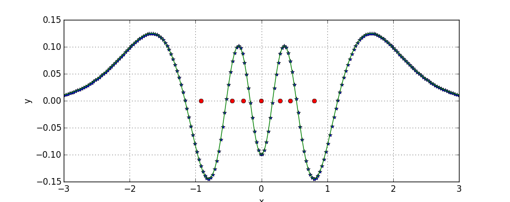
First I would like to demonstrate on a more abstract level that when the number of smaller models consisting one big model is increased learning with such model becomes easier. Consider for example the task of fitting data points shown on the following figure:

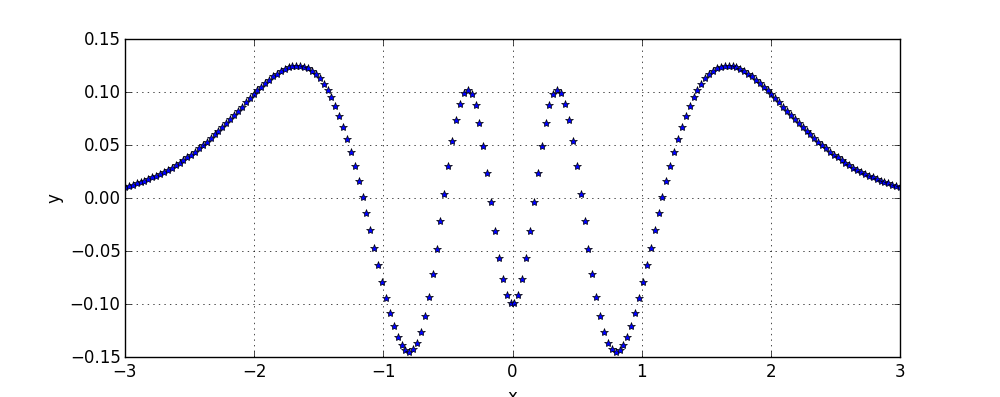
Consider using a model consisting of a single Gaussian. Such model has only 2 parameters: mean and deviation. It is computationally tractable to perform a brute force search over parameters and thus to recover the best possible placement of the Gaussian:

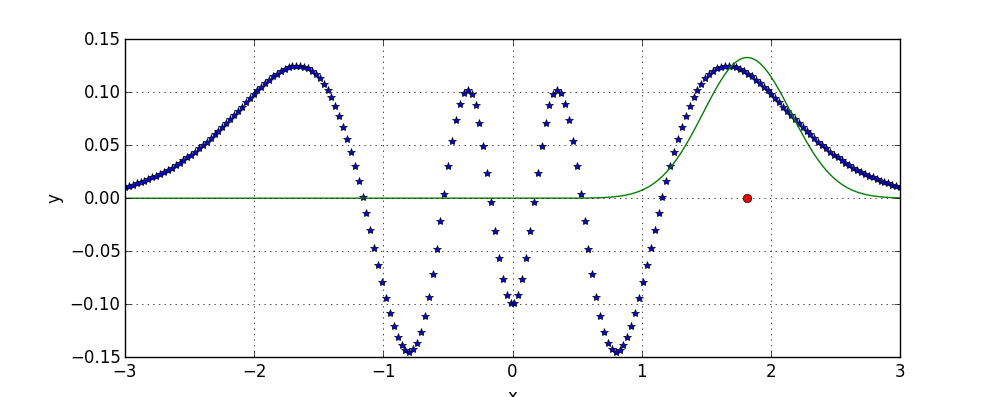
In the above figure and in the next ones, red dot denotes the mean of the Gaussian.

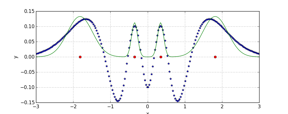
Now consider that instead of one Gaussian our model is a sum of four Gaussians. As the number of parameters of our model increases, a simple approach of enumeration rapidly becomes intractable, and thus methods like gradient descent are used instead, which frequently lead to a local minimum. For example, the following model is example of a local minimum achieved with the gradient descent:

while the globally optimal arrangement of four Gaussians fits the data perfectly:

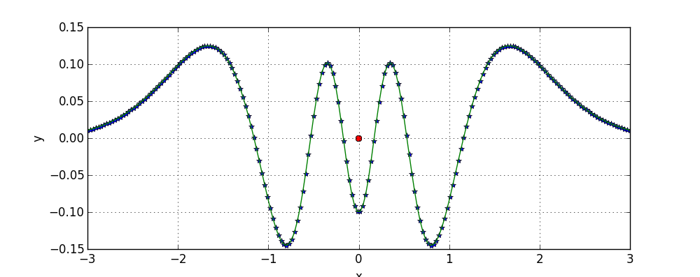
In the above figure there are four Gaussians with the same mean, that is why there appear to be only one red dot.

Above example show that a local minimum can be much worse than the global optimum.

As the number of Gaussians consisting our model further increases, so does the number of local minimum’s that gradient descent can converge to. However, as you get more Gaussians to fit your data, it becomes harder to fit the data badly. In the previous example of bad local minimum, if you would have some extra Gaussians at your disposal you could “fix” bad areas of local minimum. Adding such extra Gaussians to the initialization that lead to the mentioned bad local minimum yields:

which is in fact equal to the global optimum.

Furthermore, you could think of some simple strategies on how to train a model given unlimited Gaussians such that you are guaranteed that you will not arrive at a “bad” model. For example, you can add a Gaussian to the place in your data where model and data disagree most; You repeat this procedure until difference between the data and model is below some threshold, or when the cross validation error starts to grow.

An extreme example of such strategies is when every point in your dataset has a separate Gaussian. For every such Gaussian you set its deviation to be infinitesimally small so that it does not overlap with other Gaussians, and its height to be equal to the value of the data, and voilà! You don’t even need training for your model, and you fit your data perfectly. Needles to say though, how bad such model would overfit.

Definition of Learning Problem

In order to proceed, I first specify a widely used formulation of training of the neural network as an optimization problem.

I assume that some data is given in the form of the matrix \(X \in R^{n \times m}\) (locations of data points) and a vector \(Y \in R^{n} \) (values to fit at points \(X\)). Outputs of such network for every training point I write as \( f(X, W) \to R^{n} \), with net parameters denoted as \( W \in R^{k} \). I formulate the learning problem in the vector form as the following optimization problem:

$$\min\limits_{W \in R^{k}} || f(X,W) - Y ||_2^2\label{eq:main}$$

Shallow Networks: in Between Two Extremes

We start with shallow networks, properties of which we will use to show some interesting things for deep networks.

Shallow network consists of a single layer of hidden neurons. Let the output of neuron for some input \( x \in R^{m} \) and its parameters \( w \in R^{m} \) be denoted as a function \( g(x,w) \to R \). I define the output of a shallow network for some input \(x \in R^{m} \) to be a linear combination of \(u\) neuron outputs:

$$f(x,W) = \sum_{i \in 1 ... u} g_i(x,w_i) s_i$$

where values of \( w_i \) and \(s_i\) are stored in the vector \(W\).

Due to the way the output of the shallow neural network is computed its training is a non-convex optimization problem. Due to this property, training of a neural network suffer from the local minimum problem.

For convenience, let \(G \in R^{n \times u} \) denote separate outputs of neurons for every training point in our dataset.

Imagine that I fix parameters of every of \(m\) neurons of the shallow network. Then the training optimization problem specifies to:

$$\min\limits_{s \in R^{u}} || G s - Y ||_2^2 \label{eq:lin-fxnn}$$

All of a sudden, the learning problem becomes convex! This means that it can always be solved to the global optimality with the gradient descent over \(s \in R^{u}\). Moreover, its solution is always an upper bound on any local minimum of the original training problem achieved from fixed weights of the network. This means that if we are able to give some upper bound on a solution of above problem, it will hold for the non-convex one.

There are two extreme cases for shallow neural networks with fixed neurons, which define how bad / good such networks can fit the data.

In general, you can always set vector \(s\) to be all zeros, and then the worst objective value of \(\eqref{eq:lin-fxnn}\) would be the sum of squared values of data points - \( ||Y||_2^2 \). Furthermore, if a bias can be additionally added to the expression inside the norm in \(\eqref{eq:lin-fxnn}\), the worst objective becomes sum of squared deviations of data values from the mean.

On the other side, consider a case when the number of neurons is equal to the number of data points. Then \(G\) becomes a square matrix. Given that the determinant of \(G\) is non zero (which will be shown to hold in practice), solution to \(\eqref{eq:lin-fxnn}\) can be found by simply solving a system of linear equations \(G s = Y\). This in turn means that the objective value for a solution \(s\) would be zero. As this is an upper bound on the non-convex problem \(\eqref{eq:main}\), and as its objective always greater equal than zero, this implies that \(s\) together with fixed neuron parameters is a globally optimal solution to \(\eqref{eq:main}\). Again, such neural network would overfit the data beyond anything imaginable (recall the same scenario in the previous section).

For the number of neurons in between 0 and \(|X|\) (size of the dataset) the values will be distributed in between \( ||Y||_2^2 \) and 0 correspondingly. It is however not clear how “even” these values are distributed with respect to the number of neurons used.

First, I show that adding extra neurons with fixed parameters to the network always improves the objective value, given that randomly initialized neurons satisfy a certain criterion (which happens with probability close to / almost 1, depending on the type of neuron), outlined below.

Theorem 1. Given \(u\) neurons, adding one extra neuron to the network improves the objective \(\eqref{eq:lin-fxnn}\) if and only if it does not hold that

$$g'^T Gs = g'^T Y$$

where \(g’\) are output values of the added neuron for every training point.

Proof of the theorem is in the end of the post.

Observe that above equation defines some linear subspace of \(R^{n}\). Given some point \(g’\) uniformly sampled from \(R^{n}\), probability of “hitting” such subspace is almost zero. In practice outputs are not uniform, and belong to some non-linear subspace defined by all possible outputs of the neuron for training points. One can argue that due to the non-linearity of neurons it would still be “hard” to hit the linear space. In order to keep things simple, I verify such claim experimentally with the artificial data. Python code that can be used to reproduce experiments below is in my github repository. Experimental results shown below are for a simple artificial problem of fitting 100 values of the 2d function with a different number of neurons.

First I try neurons with the tanh non-linearity. As the hyperbolic tanhent is non-linear almost everywhere, I expect that due to this property the space where the output \(g \in R^{n}\) lives is also non-linear almost everywhere, and thus “hitting” its intersection with the linear subspace is almost impossible. Indeed, for around 10000 extensions of the random neural network of size 1 - 100 neurons its objective did not improve only once (and it might have happened due to numerical errors).

A different story is for the ReLU non-linearity, which is linear almost everywhere except for 0. For 15000 added neurons 5000 did not improve the objective function. This is due to sampled weights being too large, which results in many of 5000 neurons either returning 0 or being completely linear for all data points. In order to avoid that, I multiplied sampled weights by 0.01, which reduced the number of non-improving neurons to 1000. It appears that due to ReLU neurons being “more linear”, it is easier to “hit” the linear subspace. Nevertheless, for a proper sampling of weights such probability is small.

Above results suggest that a network can be extended by some random neuron such that it would yield an improvement of the objective with some large probability.

It is however not clear how much extra neurons improve the objective. To gain some insight, consider average objective values for the described supervised pretraining, with dataset of 100 training points (here and below similar as in previous experiment) and a different number of neurons. Here the tanh non-linearity was used. Results were averaged over one hundred different random instances of dataset.

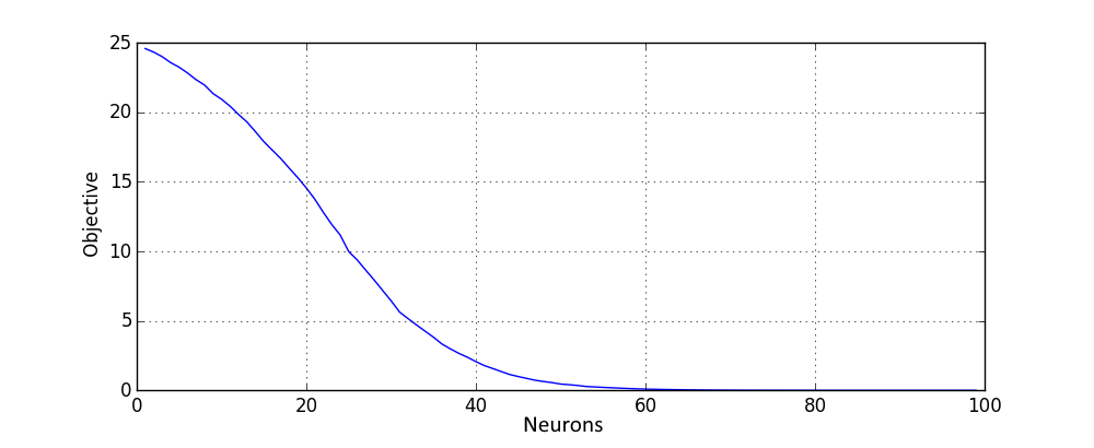
All of above values of objective function are upper bounds on any local minimum of \( \eqref{eq:main} \), which bounds how “bad” a local minimum could be. This confirms our theoretical derivations for shallow networks and demonstrates that the local minimum quality, as measured by the objective function, rapidly improves with the increase of the number of neurons. In order to see better how objective behaves for a larger amount of neurons, here is the same plot on the logarithmic scale:

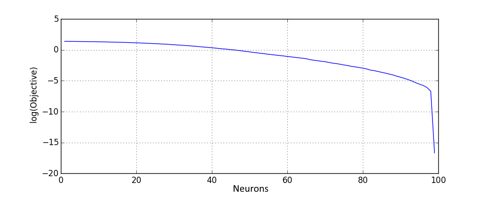
As expected, when the number of neurons approach the size of dataset, objective rapidly approaches zero.

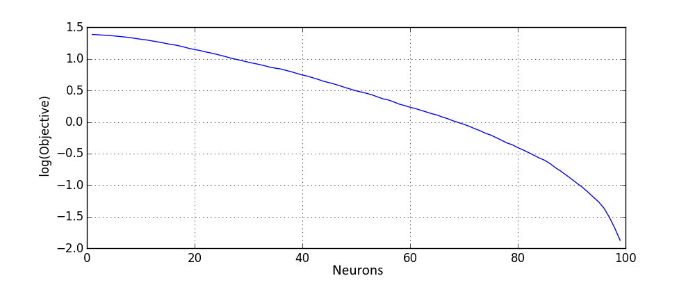
Here are similar results for the rectified linear activation, where only neurons that improve the objective were used for the network extension:

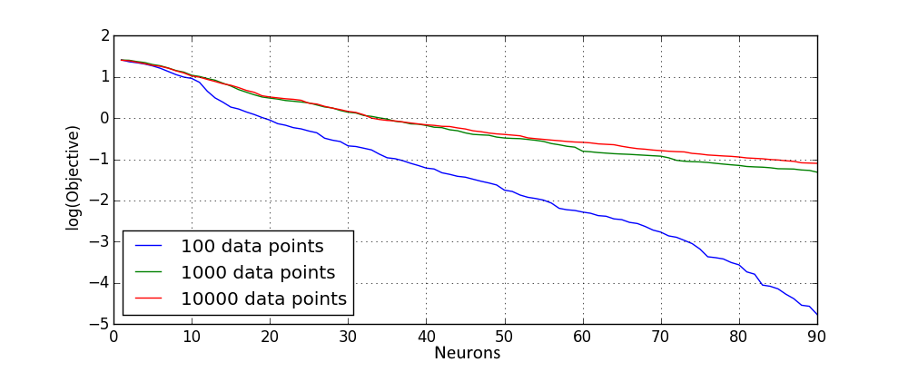
It is also interesting to see how such the distribution of upper bounds changes with dataset size. This can be seen on the following figure, where different dataset size was used and objective values were scaled in order to make results comparable:

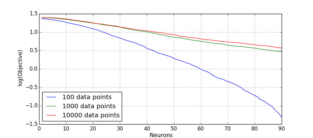
One can see that due to small dataset size model for 100 points overift, which results in much smaller values of objective for the small dataset. However for larger dataset sizes small number of neurons yield almost the same scaled objective value. This is expected, as it is generally assumed that the “complexity” of the ground truth does not change with the increased size of the dataset, and as one has enough data in order for the model to generalize well, the average “error” (scaled objective) of the model should generalize for the extra data as well.

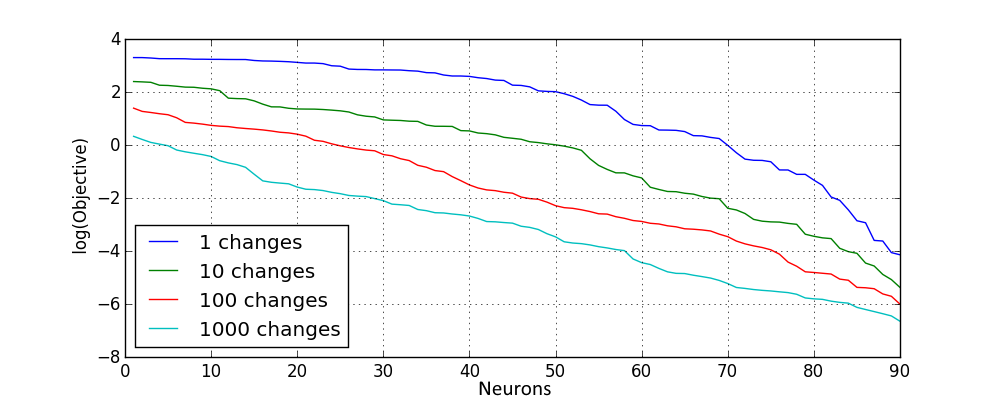
One can think of different ways on how to improve the initialization of the network so that it results in better objective values. For example, multiple neuron “candidates” can be sampled and the one is selected which yields the best objective improvement. What I however found more efficient is after every neuron addition make some random changes to the network weights and save the change if it leads to objective improvement. With a larger number of changes I get better results, summarized in the following plot for the tanh non-linearity:

Similar results are obtained for the rectified linear activation:

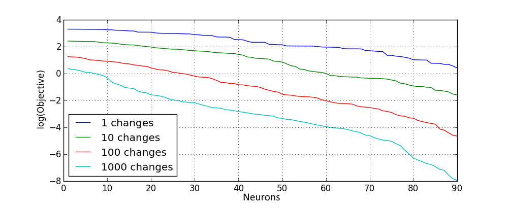
This shows that with more advanced random pretraining procedures it is possible to improve the initialization and obtain a better guarantee on a local minimum. Such procedure would be used as well in the next section, where for deep network quality of outputs of a deeper layer depend greatly on the quality of the previous layer. Furthermore, using only such procedure already at pretraining phase models with low objective value can be obtained:

The mean squared error can be calculated from objective values in above plot by dividing them by 100. So, the best mean squared error obtained for models that do not overfit is around 1e-3.

Extra Layers for Error Correction

Imagine that you trained your shallow neural net with fixed neuron parameters, but you are not satisfied with the objective value you are getting. Instead of adding additional neurons or optimizing over neuron parameters, you want to add an extra layer in order to improve the network performance. Thus adding an extra layer(s) to the network should perform an “error correction” of the previous layers of the network.

Before I proceed note that here I still fix all of the neuron parameters. This allows to write extension of a network by one layer in a very simple way by setting \(X\) equal to \(G\), and setting as \(G\) the outputs of neurons of a new layer on updated \(X\). Also for simplicity I assume that the number of neurons is similar on each layer of the (now deep) network. Similar to the previous section, an objective value for the initialization with fixed neurons parameters yields an upper bound on a local minimum achieved from such initialization with a gradient descent.

How do you correct errors? First you make sure that you do not create any extra ones! For a neural net this means that extending the network by a one more layer should be done in such a way that is is guaranteed that the objective value of a network does not increase.

One way to do this as follows. Let \(s \in R^{u}\) denote weights of optimal linear combination for outputs of previously deepest hidden layer now denoted as \(X\). By adding a neuron with the linear activation function \(g(x) = x^T s\) to the new layer we necessary preserve the objective value, as weight for such neuron is necessary selected in the best way possible due to convexity of \(\eqref{eq:main}\). This means that a weight can be set to one for the linear activation neuron and zero for all other neurons in the layer, which would necessary yield the objective of the network before the extension.

Above trick guarantees that extra layers necessary do not degrade the value of the objective function. This together with results associated with Theorem 1 in the previous section suggests that adding an extra layer would improve the value of the objective function with high probability.

Lets do some experimental verification. I start with an experiment where the network is extended a number of times by the layer consisting of one neuron with the rectified linear activation and one linear neuron as per described trick. Every time I add one extra neuron, I perform 100 iterations of random permutation procedure described in the previous section on every extra layer in order to improve its quality. Results are averaged over 10 instances of dataset used in the previous section and they look as follows:

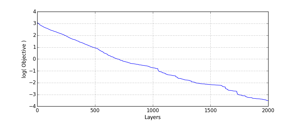
Extending the network by extra layers allows to steadily decrease the objective value as expected, even though for the deep case I cannot state the bound on the number of neurons when the objective would turn to zero. Wider networks should allow to perform better corrections and thus with a larger number of neurons in layers objective should improve faster. This is confirmed by following results with 5 ReLU neurons:

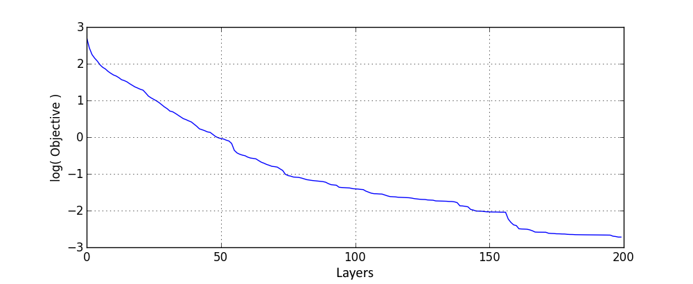
Results are similar to ones with one ReLU, except that here 10 times less layers were used.

It appears that already with the described supervised pretraining for a deep network, objective value of an arbitrary quality can be achieved, when the number of layers is not fixed. It is not clear however for which number of layers objective would turn to zero and if there might exist some dataset for which objective would never turn to zero. However I will show below that deep fully connected network can be modified such that guarantees similar to shallow networks can be given.

One of the issues I expected from deep nets is the following: it might happen that an information that is passed through layers is scrambled to such extend by all of the processing that a further error correction yields very small to none improvements of the objective function (that is also another reason I used random permutations to improve layer quality). One way to avoid this explicitly it to connect every additional layer to the input layer, so that it always has access to the “unscrambled” input. Here are results with 5 ReLU neurons:

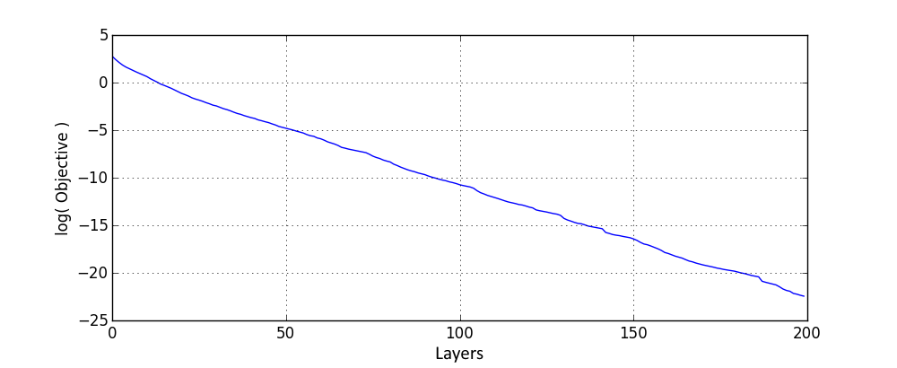
Indeed, compared to the network with no connection of deeper layers to input, the network objective improves much faster.

What is more interesting is that such a deep network can be constructed from a shallow network as follows: let \(l\) be the number of layers, and \(n\) be the number of neurons in the layer. First, pretrain a shallow network with \(l n\) neurons as in the previous section (optionally, you can also do the gradient descent after initialization). Then, select first \(l\) neurons of a shallow net with output weights \(s\), and add them as a first layer of the deep network. Add the next layer; To the deepest layer add a neuron with the linear activation which corresponds to \(f(x) = s^T x\) and next \(l\) neurons of a shallow net and set \(s\) to their output weights. Add one more layer. To the deepest layer add a linear neuron which has weights \(s\) for ReLU neurons on the previous layers and 1 for the linear activation neuron. Recursively apply the above procedure, until all of neurons of a shallow net are used. Set as output of network linear combination of outputs of the last layer, where weights of ReLU’s correspond to weights in the shallow network and weight of linear neuron is 1.

As such deep net is constructed from shallow one, this means that all of the analysis in the previous section applies to such network! Furthermore, it is guaranteed that such deep architecture would perform as good as the shallow network that it was constructed from.

It might not always be practical to connect all layers to the input layer, as input size can be large, which would increase greatly the number of parameters in a network and thus make it more prone to overfitting. One way to avoid this is instead of connecting to the input, deeper layers can connect to the first layer after the input, which can be made to have a smaller number of outputs compared to size of an input. One can think of many other ways to connect deeper layers to the ones close to the input. Somewhat similarly it was shown that connecting output layer to the ones close to input helps with network training.

Conclusion

Indeed, as the size of neural network grows, learning becomes less sensitive to the local minimum problem. This was demonstrated for both shallow and deep neural networks using a supervised pretraining procedure, which allows to obtain any desired objective value, given that number of neurons / layers is not fixed, and which provides an upper bound on any local minimum objective value.

Computational power accessible to regular user grows exponentially by Moore’s law. This means that using large neural networks becomes quickly feasible for “machine learning in the wild”, and as convergence to a local minimum becomes less of a problem for big networks this means that their training should only become more efficient, which would contribute to further success of deep learning.

Proof of Theorem 1

Let \(s’\) denote a weight for a newly added neuron. The objective function with one extra neuron is

$$|| \left(\begin{array}{cc} g' & G \end{array} \right) \left( \begin{array}{cc} s' \\\\ s \end{array} \right) - Y||_2^2$$

At the optimum of the L2 regression optimization problem it holds that:

$$\left( \begin{array}{cc} g' & G \end{array} \right)^T ( \left( \begin{array}{cc} g' & G \end{array} \right) \left( \begin{array}{cc} s' \\\\ s \end{array} \right) -Y) = 0$$

This alternatively can be written as

$$\left( \begin{array}{cc} g'^T g' & g'^T G \\\\ G^T g' & G^T G \end{array} \right) \left( \begin{array}{cc} s' \\\\ s \end{array} \right) = \left( \begin{array}{cc} g'^T Y \\\\ G^T Y \end{array} \right)$$

If neuron being added does not allow to improve the objective value, then setting \(s’\) to zero and \(s\) to weights before the network was extended should satisfy above system of equations due to the convexity of the optimization problem. For selected value of \(s\) and \(s’\) it holds that the only equation that does not necessary holds is

$$g'^T Gs = g'^T Y$$

Thus, if above equation does not hold, then the gradient of objective for \(s’ = 0\) is non zero, and thus objective can be improved at least a little bit.